Raytracing with inclination

This example shows how to access coordinate information from the raytracing process. You will likely need to do this when making custom physics materials. We will raytrace a sequence of cones in the region around a Kerr black hole as seen by an observer stationed at infinity. We will show the emission coordinates of the n=0 (direct) and n=1 (indirect) photons that are emitted from the source, at a fixed inclination angles with respect to the black hole's spin axis.

First, let's import Krang and CairoMakie for plotting.

using Krang
using CairoMakie

curr_theme = Theme(
    Axis = (
        xticksvisible = false,
        xticklabelsvisible = false,
        yticksvisible = false,
        yticklabelsvisible = false,
        aspect=1
        ),
    Heatmap = (
        rasterize=true,
    )
)
set_theme!(merge!(curr_theme, theme_latexfonts()))

We will use a 0.99 spin Kerr black hole viewed by an asymptotic observer at an inclination angle of θo=π/4. A region spanned by radii between the horizon and 10M at varying inclinations will be raytraced onto the 15x15 screen of the observer.

metric = Krang.Kerr(0.99); # Kerr metric with a spin of 0.99
θo = 45 * π / 180; # inclination angle of the observer. θo ∈ (0, π)
sze = 400; # resolution of the screen is sze x sze
rmin = Krang.horizon(metric); # minimum radius to be raytraced
rmax = 10.0; # maximum radius to be raytraced
ρmax = 15.0; # horizontal and vertical limits of the screen

Create Figure

fig = Figure(resolution=(700, 700));
axes_list = [
    [
        Axis(fig[i, 1], title=(i==1 ? "Regularized Time" : ""), titlesize=20, ylabel=(i==1 ? L"n=0" : i==2 ? L"n=1" : L"n=2"), ylabelsize=20),
        Axis(fig[i, 2], title=(i==1 ? "Radius" : ""), titlesize=20),
        Axis(fig[i, 3], title=(i==1 ? "Azimuth" : ""), titlesize=20),
    ] for i in 1:3
]

3-element Vector{Vector{Makie.Axis}}:
 [Axis (0 plots), Axis (0 plots), Axis (0 plots)]
 [Axis (0 plots), Axis (0 plots), Axis (0 plots)]
 [Axis (0 plots), Axis (0 plots), Axis (0 plots)]

Initialize Camera and pre-allocate memory for data to be plotted

coordinates = (zeros(sze, sze) for _ in 1:3)
camera = Krang.SlowLightIntensityCamera(metric, θo, -ρmax, ρmax, -ρmax, ρmax, sze);
colormaps = (:afmhot, :afmhot, :hsv)
colorrange = ((-20, 20), (0, rmax), (0, 2π))

((-20, 20), (0, 10.0), (0, 6.283185307179586))

Let's define a function that will return the coordinates of a ray when it intersects with a cone of opening angle ${\theta }_s$. We will includes some basic occlusion effects by checking if the ray intersects with the cone on the 'far-side' or the 'near-side'.

function coordinate_point(pix::Krang.AbstractPixel, geometry::Krang.ConeGeometry{T,A}) where {T, A}
    n, rmin, rmax = geometry.attributes
    θs = geometry.opening_angle

    coords = ntuple(j -> zero(T), Val(4))

    isindir = false
    for _ in 1:2 # Looping over isindir this way is needed to get Metal to work
        isindir ⊻= true
        ts, rs, θs, ϕs =  emission_coordinates(pix, geometry.opening_angle, isindir, n)
        if rs ≤ rmin || rs ≥ rmax
            continue
        end
        coords = isnan(rs) ? observation :  (ts, rs, θs, ϕs)
    end
    return coords
end

coordinate_point (generic function with 1 method)

Draw Function This function draws the coordinates associated with the n=0,1,2 subimages of a cone with opening angle θs.

function draw!(axes_list, camera, coordinates, rmin, rmax, θs)
    times, radii, azimuths = coordinates
    map(axes -> empty!.(axes), axes_list)

    geometries = (Krang.ConeGeometry(θs, (i, rmin, rmax)) for i in 0:2)

    for (i, geometry) in enumerate(geometries)
        rendered_scene = coordinate_point.(camera.screen.pixels, Ref(geometry))
        for I in CartesianIndices(rendered_scene)
            times[I] = rendered_scene[I][1]
            radii[I] = rendered_scene[I][2]
            azimuths[I] = rendered_scene[I][4]
        end
        coordinates = (times, radii, mod2pi.(azimuths ))
        for j in 1:3
            heatmap!(axes_list[i][j], coordinates[j], colormap = colormaps[j], colorrange=colorrange[j])
        end
    end
end

draw! (generic function with 1 method)

Create the animation of Cone of Emission Coordinates

recording = CairoMakie.record(fig, "coordinate.gif", range(0.0, π, length=180), framerate=12) do θs
    draw!(axes_list, camera, coordinates, rmin, rmax, θs)
end

"coordinate.gif"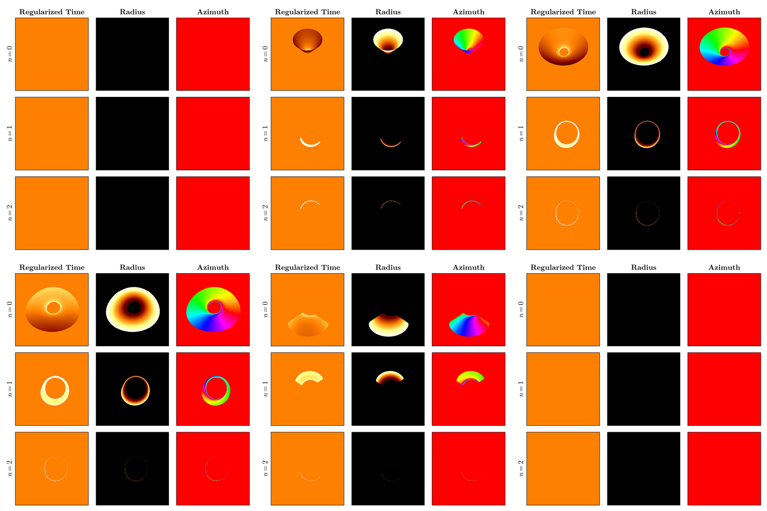

The GPU can be used in this example with an appropriate broadcast.

using CUDA

rendered_scene = Array(coordinate_point.(CuArray(camera.screen.pixels), Ref(geometry)))

---

This page was generated using Literate.jl.