Rays & Coordinate information with Mino time (τ)

In this example, we will ray trace the region around a Kerr black hole as seen by an observer stationed at infinity. We will return the coordinates associated with a ray by marching along the ray's Mino time parameter from the assymptotic observer. This information can be easily accessed using the emission_coordinates! function.

Setup

First, let's import Krang and CairoMakie for plotting.

using Krang
import GLMakie as GLMk
GLMk.Makie.inline!(true)

curr_theme = GLMk.Theme(# Makie theme
    fontsize = 20,
    Axis = (
        xticksvisible = false,
        xticklabelsvisible = false,
        yticksvisible = false,
        yticklabelsvisible = false,
        leftspinevisible = false,
        rightspinevisible = false,
        topspinevisible = false,
        bottomspinevisible = false,
        titlefontsize = 30,
    ),
)

GLMk.set_theme!(GLMk.merge(curr_theme, GLMk.theme_latexfonts()))

We will use a 0.99 spin Kerr black hole viewed by an asymptotic observer at an inclination angle of θo=π/4.

metric = Krang.Kerr(0.99); # Kerr spacetime with 0.99 spin
θo = 85 * π / 180; # Observer inclination angle with respect to spin axis
sze = 200; # Number of pixels along each axis of the screen
ρmax = 5; # Size of the screen

We will define a camera with the above parameters. The `SlowLightIntensityCamera`` pre-calculates information about the spacetime and the observer's screen to speed up the raytracing for slow light applications.

camera = Krang.SlowLightIntensityCamera(metric, θo, -ρmax, ρmax, -ρmax, ρmax, sze);

Plotting coordinates

We will create a loop to plot the emission coordinates for each τ using the emission_coordinates! function. Let us now create a figure to plot the emission coordinates on.

fig = GLMk.Figure(size = (500, 600));


recording =
    GLMk.record(fig, "raytrace.gif", range(0.1, 3, length = 290), framerate = 15) do τ
        GLMk.empty!(fig)

        coordinates = zeros(4, size(camera.screen.pixels)...) # Pre allocated array to store coordinates
        emission_coordinates!(coordinates, camera, τ)
        time = coordinates[1, :, :]
        radius = coordinates[2, :, :]
        inclination = coordinates[3, :, :]
        azimuth = mod2pi.(coordinates[4, :, :])

        data = (time, radius, inclination, azimuth)
        titles = (
            GLMk.L"\text{Regularized Time }(t_s)",
            GLMk.L"\text{Radius }(r_s)",
            GLMk.L"\text{Inclination }(\theta_s)",
            GLMk.L"\text{Azimuth } (\phi_s)",
        )
        colormaps = (:afmhot, :afmhot, :afmhot, :hsv)
        colorrange = ((-20, 20), (0, 10.0), (0, π), (0, 2π))
        indices = ((1, 1), ())

        for i = 1:4
            hm = GLMk.heatmap!(
                GLMk.Axis(
                    getindex(fig, (i > 2 ? 2 : 1), (iszero(i % 2) ? 3 : 1));
                    aspect = 1,
                    title = titles[i],
                ),
                data[i],
                colormap = colormaps[i],
                colorrange = colorrange[i],
            )
            cb = GLMk.Colorbar(
                fig[(i > 2 ? 2 : 1), (iszero(i % 2) ? 3 : 1)+1],
                hm;
                labelsize = 30,
                ticklabelsize = 20,
            )
        end

        ax = GLMk.Axis(fig[3, 1:3], height = 60)
        GLMk.hidedecorations!(ax)
        GLMk.text!(ax, 0, 100; text = GLMk.L"θ_o=%$(Int(floor(θo*180/π)))^\circ")
        GLMk.rowgap!(fig.layout, 1, GLMk.Fixed(0))
    end

"raytrace.gif"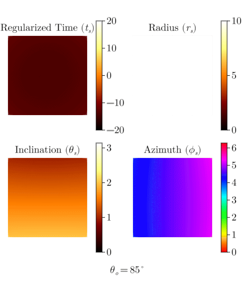

Plotting rays

Let's also plot the rays that are traced from the screen to the observer. Rays can be generated using the generate_ray function.

We will plot a ray for each pixel in the camera.

camera = Krang.SlowLightIntensityCamera(metric, θo, -3, 3, -3, 3, 4);

fig = GLMk.Figure()
ax = GLMk.Axis3(fig[1, 1], aspect = (1, 1, 1))
GLMk.xlims!(ax, (-3, 3))
GLMk.ylims!(ax, (-3, 3))
GLMk.zlims!(ax, (-3, 3))
lines_to_plot = []
lines_to_plot = Krang.generate_ray.(camera.screen.pixels, 5_000)

sphere = GLMk.Sphere(GLMk.Point(0.0, 0.0, 0.0), horizon(metric))
GLMk.mesh!(ax, sphere, color = :black) # Sphere to represent black hole

for i in lines_to_plot
    ray = map(x -> begin
        (; rs, θs, ϕs) = x
        [rs * sin(θs) * cos(ϕs), rs * sin(θs) * sin(ϕs), rs * cos(θs)]
    end, i)
    ray = hcat(ray...)
    GLMk.lines!(ax, ray)
end
fig

GLMk.save("mino_time_rays.png", fig)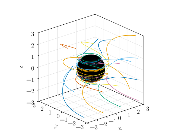

---

This page was generated using Literate.jl.