Creating a Custom Dual Cone Model

We will define a custom model for low luminosity active galactice nuclei (LLAGN). A detailed description of the model can be found in this reference. We will show the emission of the n=0 (direct) and n=1 (indirect) photons as they are emitted from the source, at a fixed inclination angle from the black hole's spin axis.

First, let's import Krang and CairoMakie for plotting.

using Krang
using CairoMakie

curr_theme = Theme(
    Axis = (
        xticksvisible = false,
        xticklabelsvisible = false,
        yticksvisible = false,
        yticklabelsvisible = false,
    ),
)
set_theme!(merge!(curr_theme, theme_latexfonts()))

We will use a $0.94$ spin Kerr black hole viewed by an asymptotic observer at an inclination angle of $\theta o={17}^{\circ }$. The emission to be ray traced is

metric = Krang.Kerr(0.94);
θo = 17 * π / 180;
ρmax = 10.0;

Let's create a camera with a resolution of 400x400 pixels

camera = Krang.IntensityCamera(metric, θo, -ρmax, ρmax, -ρmax, ρmax, 400);

We will need to create Mesh objects to render the scene. First we will create the material for the mesh. Our material will be the ElectronSynchrotronPowerLawPolarization material with the following parameters.

χ = -1.705612782769303
ι = 0.5807355065517938
βv = 0.8776461626924748
σ = 0.7335172899224874
η1 = 2.6444786738735804
η2 = π - η1

0.49711397971621274

These will be used to define the magnetic field and fluid velocity.

magfield1 = Krang.SVector(sin(ι) * cos(η1), sin(ι) * sin(η1), cos(ι));
magfield2 = Krang.SVector(sin(ι) * cos(η2), sin(ι) * sin(η2), cos(ι));
vel = Krang.SVector(βv, (π / 2), χ);
R = 3.3266154761905455
p1 = 4.05269835622511
p2 = 4.411852974336667

4.411852974336667

Next we will define the geometries of each mesh. We will use a ConeGeometry with an opening angle of ${75}^{\circ }$. The additional information needed for the material will be passed as attributes to the geometry. This includes the sub-images to ray trace, which in our case will be the n=0 and n=1 sub-images.

θs = (75 * π / 180)
material1 = Krang.ElectronSynchrotronPowerLawPolarization(
    magfield1...,
    vel...,
    σ,
    R,
    p1,
    p2,
    (0, 1),
);
geometry1 = Krang.ConeGeometry((θs))
material2 = Krang.ElectronSynchrotronPowerLawPolarization(
    magfield2...,
    vel...,
    σ,
    R,
    p1,
    p2,
    (0, 1),
);
geometry2 = Krang.ConeGeometry((π - θs))

Krang.ConeGeometry{Float64, Nothing}(1.832595714594046, nothing)

We will create two meshes, one for each geometry anc create a scene with both meshes.

mesh1 = Krang.Mesh(geometry1, material1)
mesh2 = Krang.Mesh(geometry2, material2)

Krang.Mesh{Krang.ConeGeometry{Float64, Nothing}, Krang.ElectronSynchrotronPowerLawPolarization{2, Float64}}(Krang.ConeGeometry{Float64, Nothing}(1.832595714594046, nothing), Krang.ElectronSynchrotronPowerLawPolarization{2, Float64}([0.4822331381486707, 0.2616409108851046, 0.8360593485049359], [0.8776461626924748, 1.5707963267948966, -1.705612782769303], 0.7335172899224874, 3.3266154761905455, 4.05269835622511, 4.411852974336667, (0, 1)))

Finally, we will render the scene with the camera and plot the Stokes parameters.

scene = Krang.Scene((mesh1, mesh2))
stokesvals = render(camera, scene)

fig = Figure(resolution = (700, 700));
ax1 = Axis(fig[1, 1], aspect = 1, title = "I")
ax2 = Axis(fig[1, 2], aspect = 1, title = "Q")
ax3 = Axis(fig[2, 1], aspect = 1, title = "U")
ax4 = Axis(fig[2, 2], aspect = 1, title = "V")
colormaps = [:afmhot, :redsblues, :redsblues, :redsblues]

zip(
    [ax1, ax2, ax3, ax4],
    [
        getproperty.(stokesvals, :I),
        getproperty.(stokesvals, :Q),
        getproperty.(stokesvals, :U),
        getproperty.(stokesvals, :V),
    ],
    colormaps,
) .|> x -> heatmap!(x[1], x[2], colormap = x[3])
fig

save("polarization_example.png", fig)

┌ Warning: Found `resolution` in the theme when creating a `Scene`. The `resolution` keyword for `Scene`s and `Figure`s has been deprecated. Use `Figure(; size = ...` or `Scene(; size = ...)` instead, which better reflects that this is a unitless size and not a pixel resolution. The key could also come from `set_theme!` calls or related theming functions.
└ @ Makie ~/.julia/packages/Makie/Q6F2P/src/scenes.jl:238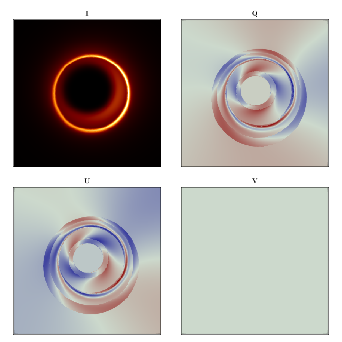

---

This page was generated using Literate.jl.