Thermal Synchrotron Disk

This example ray traces an optically thick accretion disk of thermal electrons, and shows how the image changes as the disk goes from optically thick to optically thin with increasing observing frequency.

Unlike the power law materials, Krang.ThermalSynchrotron absorbs its own emission: it reports the source function and an optical depth for each sub-image, and render solves the transfer along the ray. That is what produces the limb brightened ring below.

using Krang
import CairoMakie as CMk

curr_theme = CMk.Theme(
    Axis = (
        xticksvisible = false,
        xticklabelsvisible = false,
        yticksvisible = false,
        yticklabelsvisible = false,
        aspect = 1,
    ),
)
CMk.set_theme!(CMk.merge!(curr_theme, CMk.theme_latexfonts()))

The model

We will use parameters loosely based on M87*: a $a=15/16$ black hole of $6.5\times {10}^9{M}_{\odot }$ viewed at ${\theta }_o={17}^{\circ }$. The material works in physical units, so it needs the gravitational radius to convert the emission radius (which Krang measures in $GM/c^2$) into metres.

G = 6.6743e-11                      # m³ kg⁻¹ s⁻²
Msun = 1.988409870698051e30         # kg
rg = G * 6.5e9 * Msun / Krang.C_SI^2  # gravitational radius in metres

metric = Krang.Kerr(15 / 16);
θo = 17 * π / 180;
ρmax = 12.0;

The electron density, temperature and magnetic field each fall off as a power law in radius about a reference radius rb, and the fluid orbits with a speed of $0.5c$.

rb = 5.0                  # reference radius, in GM/c²
n_th0 = 3.0e9             # electron density at rb, m⁻³
t_e0 = 3.0e10             # electron temperature at rb, K
magnetic_field = (0.0, 8.0, 0.0)   # at rb, in Gauss
fluid_velocity = (0.5, π / 2, π / 2)
p_dens, p_temp, p_b = -0.7, -1.5, -1.5;

The disk is the ${\theta }_s=\pi /2$ cone, and we ray trace its $n=0$ and $n=1$ sub-images.

function disk(ν)
    material = Krang.ThermalSynchrotron(
        magnetic_field...,
        fluid_velocity...,
        p_dens,
        p_temp,
        p_b,
        n_th0,
        t_e0,
        rb,
        ν,
        rg,
        (0, 1),
    )
    return Krang.Mesh(Krang.ConeGeometry(π / 2), material)
end

camera = Krang.IntensityCamera(metric, θo, -ρmax, ρmax, -ρmax, ρmax, 400);

Intensity and optical depth

render hands back the intensity, but raytrace on a single mesh returns the Krang.AbsorptiveIntensity it was accumulated from, so the optical depth the ray picked up is available alongside it.

slabs = Krang.raytrace(camera, disk(230.0e9));
intensity = map(x -> x.I, slabs);
optical_depth = map(x -> x.τ, slabs);

fig = CMk.Figure(size = (850, 400));
ax1 = CMk.Axis(fig[1, 1], title = "Intensity at 230 GHz")
ax2 = CMk.Axis(fig[1, 3], title = "Optical depth at 230 GHz")
hm1 = CMk.heatmap!(ax1, intensity, colormap = :afmhot)
hm2 = CMk.heatmap!(
    ax2,
    log10.(max.(optical_depth, 1e-12)),
    colormap = :viridis,
    colorrange = (-6, 1),
)
CMk.Colorbar(fig[1, 2], hm1, label = "W m⁻² Hz⁻¹ sr⁻¹")
CMk.Colorbar(fig[1, 4], hm2, label = "log₁₀ τ")
CMk.save("thermal-disk-230.png", fig)
fig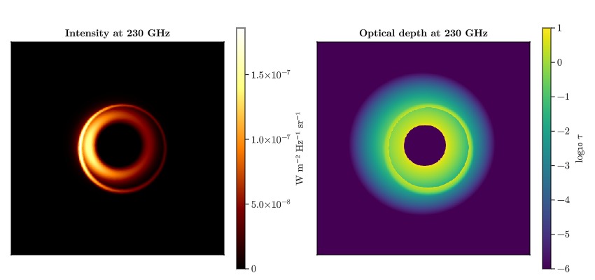

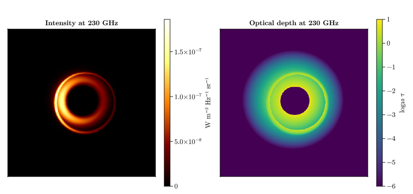
The bright ring sits where the disk becomes optically thick: only about 5% of the pixels reach $\tau >1$ here, in an annulus spanning $\rho \approx 2$ to $5GM/c^2$, and those are the ones that saturate at the source function. Rays that graze the disk travel much further through it – the obliquity factor $|p^{\hat{t}}/p^{\hat{\theta }}|$ diverges for a ray running parallel to the surface – which is what lifts the ring out of the optically thin background.

The left-right asymmetry is not an optical depth effect: the optical depth map is very nearly axisymmetric. It is Doppler beaming from the fluid, which orbits at $0.5c$, and enters through the $g^3$ factor – here a factor of $2.2$ between the approaching and receding sides.

Walking through the transition

The critical frequency ${\nu }_c\propto B{\mathrm{\Theta }}_e^2$ is fixed by the plasma, so raising the observing frequency moves the disk from optically thick to optically thin. Each panel is normalised to its own maximum so the morphology is comparable.

frequencies = (86.0e9, 230.0e9, 345.0e9, 690.0e9)
fig = CMk.Figure(size = (1000, 280));
for (i, ν) in enumerate(frequencies)
    img = render(camera, Krang.Scene((disk(ν),)))
    ax = CMk.Axis(fig[1, i], title = "$(Int(ν / 1e9)) GHz")
    CMk.heatmap!(ax, img ./ maximum(img), colormap = :afmhot, colorrange = (0, 1))
end
CMk.save("thermal-disk-frequencies.png", fig)
fig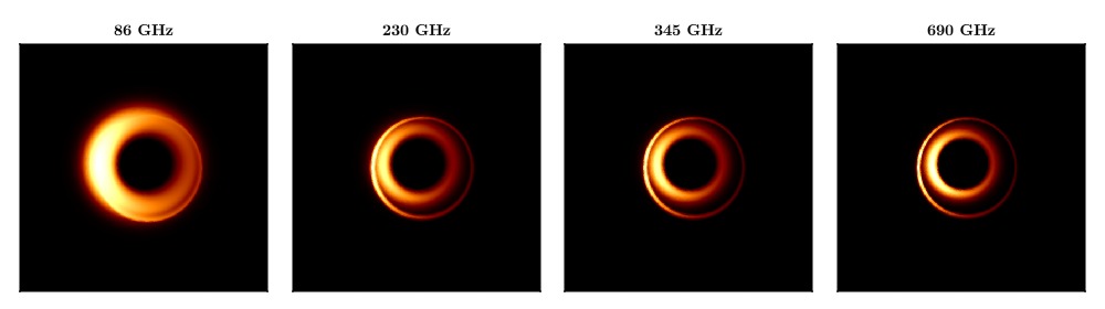

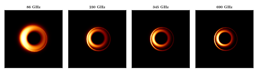
The low frequency image is a broad, saturated disk: it is optically thick out to large radii, so most rays simply return the local source function. As the frequency rises the emission narrows onto the inner disk – the horizontal cut through the centre tightens from $2.8$ to $1.3GM/c^2$ between 86 and 690 GHz, with the peak staying near $\rho \approx 4GM/c^2$ – and the sharp $n=1$ sub-image, washed out at 86 GHz, stands clear of the direct image at the high frequencies.

---

This page was generated using Literate.jl.