Neural Network Emission Model Example
This is a pedagogical example that serves as a proof of concept. We will build a simple Neural Network emission model to be ray traced and optimize with ADAM algorithm.
using Lux
using Krang
using Random
Random.seed!(123)
rng = Random.GLOBAL_RNGRandom._GLOBAL_RNG()Our model will take in spacetime coordinates and return observed intensity value for a given pixel:
We will first define a simple emisison model that will be raytraced. The emission model will ge taken to be a simple fully connected Neural Network with 2 hidden layers
emission_model = Chain(
    Dense(2 => 20, Lux.sigmoid),
    Dense(20 => 20, Lux.sigmoid),
    Dense(20 => 1, Lux.sigmoid)
    )

ps, st = Lux.setup(rng, emission_model);
We will use 0.99 spin Kerr metric with an observer sitting at 20 degrees inclination with respect to the spin axis in this example. These parameters could be made to float in the optimization process. We will do this by defining an ImageModel comprised of an emission layer and a raytracing layer. We will create a struct for our image model and store our emission model as a layer to be raytraced.
struct ImageModel{T <: Chain}
    emission_layer::T
end
The models in Lux are functors that take in features, parameters and model state, and return the output and model state.
function (m::ImageModel)(x, ps, st)
    metric = Krang.Kerr(0.99e0)
    θo = Float64(20/180*π)
    pixels = Krang.IntensityPixel.(Ref(metric), x[1,:], x[2,:], θo)

    sze = unsafe_trunc(Int, sqrt(size(x)[2]))
    coords = zeros(Float64, 2,sze*sze)
    emission_vals = zeros(Float64, 1, sze*sze)
    for n in 0:1
        for i in 1:sze
            for j in 1:sze
                pix = pixels[i+(j-1)*sze]
                α, β = Krang.screen_coordinate(pix)
                T = typeof(α)
                rs, _, ϕs = Krang.emission_coordinates_fast_light(pix, Float64(π/2), β > 0, n)[1:3]
                xs = rs * cos(ϕs)
                ys = rs * sin(ϕs)
                if hypot(xs, ys) ≤ Krang.horizon(metric)
                    coords[1,i+(j-1)*sze] = zero(T)
                    coords[2,i+(j-1)*sze] = zero(T)
                else
                    coords[1,i+(j-1)*sze] = xs
                    coords[2,i+(j-1)*sze] = ys
                end

            end
        end
        emission_vals .+= m.emission_layer(coords, ps, st)[1]
    end
    emission_vals,st
end
Lets create an 20x20 pixel image with a field of view of
image_model = ImageModel(emission_model)
sze = 20
ρmax = 10e0
pixels = zeros(Float64, 2, sze*sze)
for (iiter, i) in enumerate(range(-ρmax, ρmax, sze))
    for (jiter, j) in enumerate(range(-ρmax, ρmax, sze))
        pixels[1,iiter+(jiter-1)*sze] = Float64(i)
        pixels[2,iiter+(jiter-1)*sze] = Float64(j)
    end
end
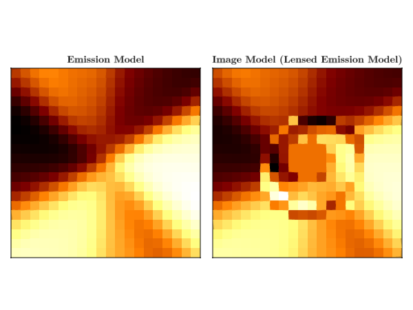
Lets see what our emission model looks like before and after raytracing.
using CairoMakie
curr_theme = Theme(
    Axis = (xticksvisible=false, xticklabelsvisible=false, yticksvisible=false, yticklabelsvisible=false,),
    Heatmap =(colormap=:afmhot, ),
)
set_theme!(merge(curr_theme, theme_latexfonts()))

emitted_intensity = reshape(emission_model(pixels, ps, st)[1], sze, sze)
received_intensity = reshape(image_model(pixels, ps, st)[1], sze, sze)

fig = Figure();
heatmap!(Axis(fig[1,1], aspect=1, title="Emission Model"), emitted_intensity)
heatmap!(Axis(fig[1,2], aspect=1, title="Image Model (Lensed Emission Model)"), received_intensity)
save("emission_model_and_target_model.png", fig)
This will be the image we will try to fit our model to.
target_img = reshape(received_intensity, sze, sze);Fitting the model
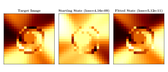
Lets fit our model using the normalized cross correlation as a kernel for our loss function.
using Enzyme
using Optimization
using OptimizationOptimisers
using StatsBase
using ComponentArrays
Enzyme.API.runtimeActivity!(true)

Enzyme.Compiler.RunAttributor[] = false

function mse(img1::Matrix{T}, img2::Matrix{T}) where T
    img1 = reshape(img1, sze, sze) ./ sum(img1)
    img2 = reshape(img2, sze, sze) ./ sum(img2)
    mean((img1 .- img2) .^ 2)
end

function loss_function(pixels, y, ps, st)
    y_pred, st = image_model(pixels, ps, st)
    mse(y, y_pred), st
end

mse(target_img, target_img)

ps, st = Lux.setup(rng, emission_model);
image_model = ImageModel(emission_model);

emitted_intensity = reshape(emission_model(pixels, ps, st)[1], sze, sze)
received_intensity = reshape(image_model(pixels, ps, st)[1], sze, sze)
loss_function(pixels, target_img, ps, st)

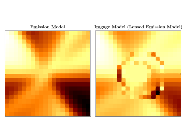
fig = Figure();
heatmap!(Axis(fig[1,1], aspect=1, title="Emission Model"), emitted_intensity, colormap=:afmhot)
heatmap!(Axis(fig[1,2], aspect=1, title="Imgage Model (Lensed Emission Model)"), received_intensity, colormap=:afmhot)
save("emission_model_and_image_model.png", fig)
WARNING: using ComponentArrays.Axis in module Main conflicts with an existing identifier.
mutable struct Callback
    counter::Int
    stride::Int
    const f::Function
end
Callback(stride, f) = Callback(0, stride, f)
function (c::Callback)(state, loss, others...)
    c.counter += 1
    if c.counter % c.stride == 0
        @info "On step $(c.counter) loss = $(loss)"
        return false
    else
        return false
    end
end

ps_trained, st_trained = let st=Ref(st), x=pixels, y=target_img

    optprob = Optimization.OptimizationProblem(
        Optimization.OptimizationFunction(
            function(ps, constants)
                loss, st[] = loss_function(x, y, ps, st[])
                loss
            end,
            Optimization.AutoEnzyme()
        ),
        ComponentArrays.ComponentVector{Float64}(ps)
    )

    solution = Optimization.solve(
        optprob,
        OptimizationOptimisers.Adam(),
        maxiters = 5_000,
    callback=Callback(100,()->nothing)
    )

    solution.u, st[]
end

received_intensity, st = ((x) -> (reshape(x[1], sze, sze), x[2]))(image_model(pixels, ps_trained, st_trained))
acc_intensity, st = ((x) -> (reshape(x[1], sze, sze), x[2]))(image_model(pixels, ps, st))
loss_function(pixels, target_img, ps, st)
loss_function(pixels, target_img, ps_trained, st_trained)
using Printf
begin
    fig = Figure(size=(700, 300));
    heatmap!(Axis(fig[1,1], aspect=1, title="Target Image"), target_img)
    heatmap!(Axis(fig[1,2], aspect=1, title="Starting State (loss=$(@sprintf("%0.2e", loss_function(pixels, target_img, ps, st)[1])))"), acc_intensity)
    heatmap!(Axis(fig[1,3], aspect=1, title="Fitted State (loss=$(@sprintf("%0.2e", loss_function(pixels, target_img, ps_trained, st_trained)[1])))"), received_intensity)
    save("neural_net_results.png", fig)
end
[ Info: On step 100 loss = 1.6055200023314324e-9
[ Info: On step 200 loss = 1.2243728625354756e-9
[ Info: On step 300 loss = 9.684756228495006e-10
[ Info: On step 400 loss = 7.732927888822727e-10
[ Info: On step 500 loss = 6.228896833155562e-10
[ Info: On step 600 loss = 5.062173801624511e-10
[ Info: On step 700 loss = 4.1436314526495676e-10
[ Info: On step 800 loss = 3.411556857185687e-10
[ Info: On step 900 loss = 2.85232287188936e-10
[ Info: On step 1000 loss = 2.4181345441538095e-10
[ Info: On step 1100 loss = 2.0783346824626142e-10
[ Info: On step 1200 loss = 1.811149772029884e-10
[ Info: On step 1300 loss = 1.600106536986751e-10
[ Info: On step 1400 loss = 1.4325779871508514e-10
[ Info: On step 1500 loss = 1.298838990123226e-10
[ Info: On step 1600 loss = 1.19138065039885e-10
[ Info: On step 1700 loss = 1.1043965204392107e-10
[ Info: On step 1800 loss = 1.0333924592964907e-10
[ Info: On step 1900 loss = 9.74888062714144e-11
[ Info: On step 2000 loss = 9.261869493559483e-11
[ Info: On step 2100 loss = 8.851993938209986e-11
[ Info: On step 2200 loss = 8.503050908129013e-11
[ Info: On step 2300 loss = 8.202468695777307e-11
[ Info: On step 2400 loss = 7.940483677970756e-11
[ Info: On step 2500 loss = 7.709502895388749e-11
[ Info: On step 2600 loss = 7.503610872290289e-11
[ Info: On step 2700 loss = 7.31818836240155e-11
[ Info: On step 2800 loss = 7.149617878527064e-11
[ Info: On step 2900 loss = 6.995056438081913e-11
[ Info: On step 3000 loss = 6.852260304774729e-11
[ Info: On step 3100 loss = 6.719449902153001e-11
[ Info: On step 3200 loss = 6.595205725895281e-11
[ Info: On step 3300 loss = 6.478388149595205e-11
[ Info: On step 3400 loss = 6.368075629211129e-11
[ Info: On step 3500 loss = 6.263517063304376e-11
[ Info: On step 3600 loss = 6.164095037626286e-11
[ Info: On step 3700 loss = 6.069297434975002e-11
[ Info: On step 3800 loss = 5.978695472890277e-11
[ Info: On step 3900 loss = 5.891926680637507e-11
[ Info: On step 4000 loss = 5.808681672818944e-11
[ Info: On step 4100 loss = 5.728693843079144e-11
[ Info: On step 4200 loss = 5.651731305857958e-11
[ Info: On step 4300 loss = 5.5775905710878206e-11
[ Info: On step 4400 loss = 5.506091557050805e-11
[ Info: On step 4500 loss = 5.437073638771706e-11
[ Info: On step 4600 loss = 5.370392499860257e-11
[ Info: On step 4700 loss = 5.305917609664002e-11
[ Info: On step 4800 loss = 5.243530188848187e-11
[ Info: On step 4900 loss = 5.183121558040993e-11
[ Info: On step 5000 loss = 5.1245917882855496e-11
This page was generated using Literate.jl.